The Assignment Was One JPEG
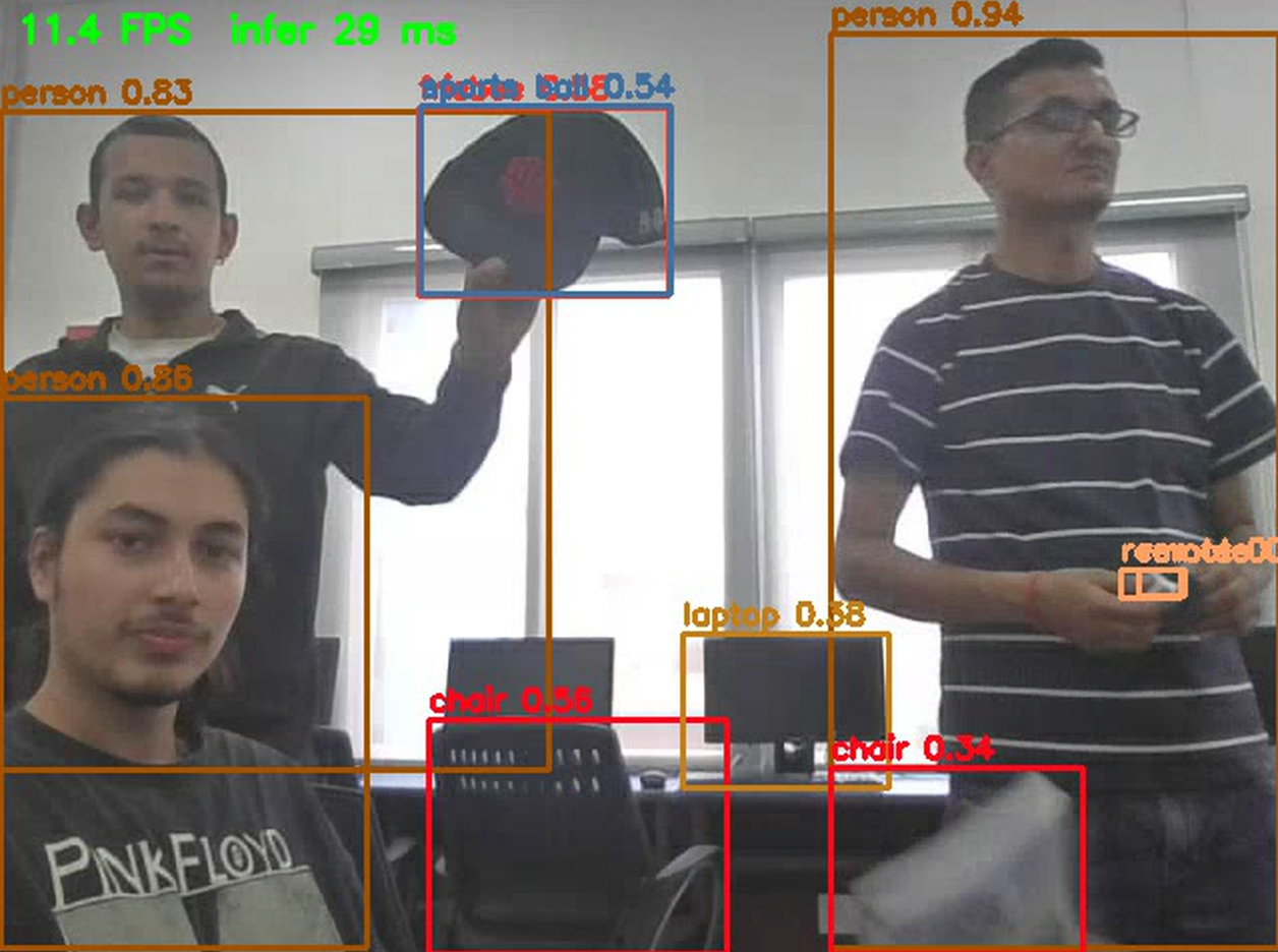
The picture at the top is a frame from the live run. The video is coming from my laptop’s webcam over the LAN, because the Nano had no camera. COCO has no class for a cap, so the model calls it a sports ball.
The assignment
This started from a short edge-computing workshop at college, spread across two days. Working in my homelab had already taught me that constrained hardware makes you notice things you can ignore on a bigger machine. You squeeze the experiment in, then try to squeeze the performance back out.
The instruction at the workshop was simple. We had an older Jetson Nano and our own laptops. Boot the board with JetPack 4.6, run a lightweight model, pass it an image, and see what it says.
I had the board for a few hours, and it belonged to someone else. By the time I handed it back, I had a TensorRT engine compiled on the board, a YOLOv8 decoder written by hand in numpy and checked against the reference, three engines benchmarked, a per-layer profile of the network, and live detection running on video from a camera the board did not even have. Then I put the board back exactly the way I found it.
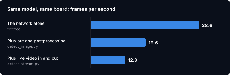
Between all this, the benchmark tool told me the model ran at 38.6 FPS. When I pointed a live camera at the same model on the same board, I got 12.3.
This blog is about where the other 26 frames per second went. The code, the raw logs and every number below are in jetson-nano-yolo-bench.
The device decides
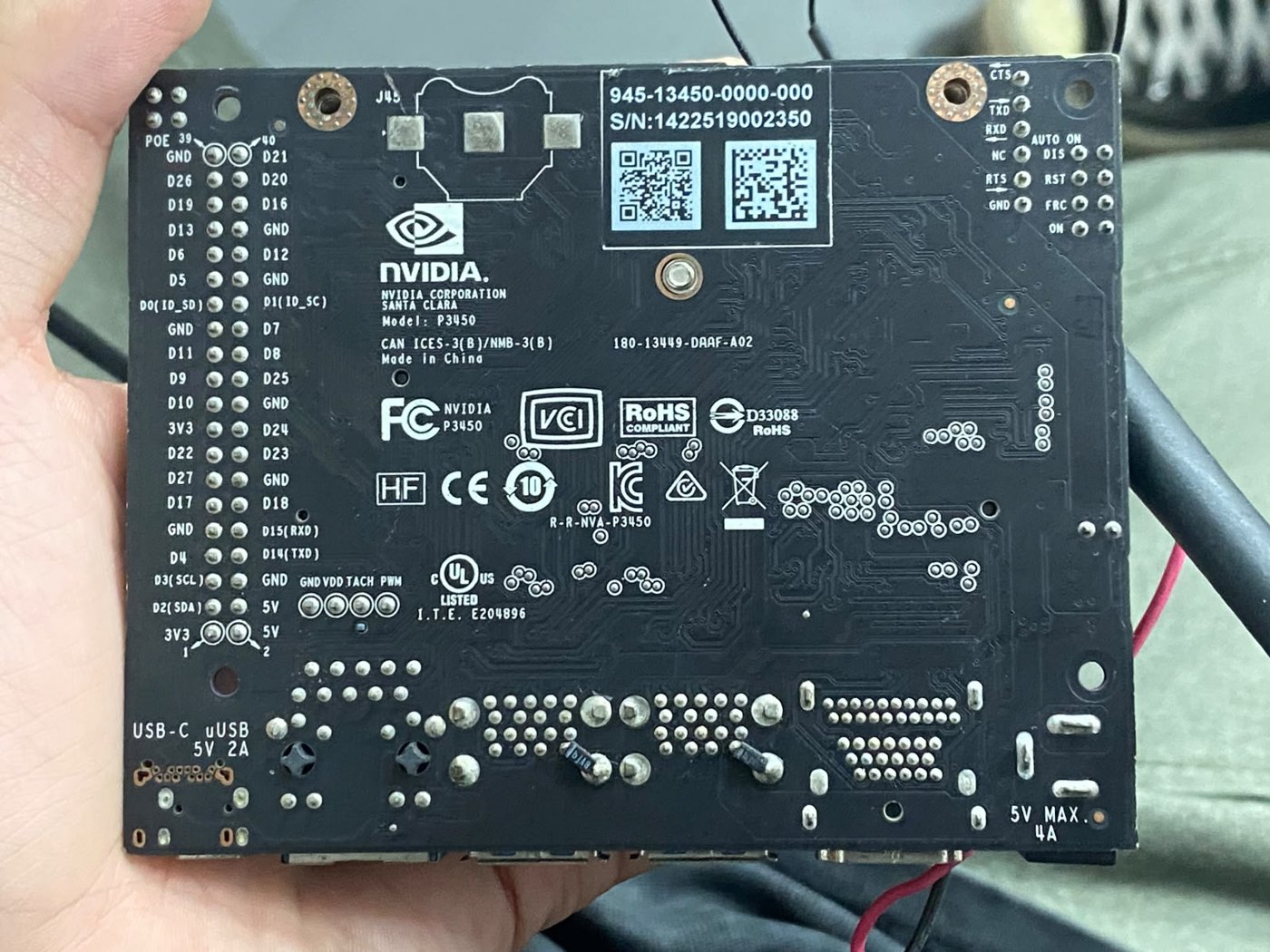
On a workstation or in the cloud, throwing more resources at a problem is often an option. More memory, a newer driver, a bigger machine. On this board it was not. The design ends up being whatever the device leaves room for, and almost every decision I made was really made by the Nano.
| Limit of the board | What it forced |
|---|---|
| JetPack 4.6 is the last release for this board, so we’re locked with Python 3.6 and TensorRT 8.0 | Export the model to ONNX on my laptop with opset=12, and send only that file to the board |
pycuda was not installed, and takes a quarter of an hour to build on the Nano |
Call cudaMalloc and cudaMemcpy from libcudart directly through ctypes. It is about ten lines |
| 4 GB of memory, shared between the CPU and the GPU, with over half taken by the desktop | Boot headless first. Idle memory use went from 2.3 GB to 276 MB |
| No camera | Stream my laptop’s webcam over the LAN and open it in OpenCV as a GStreamer pipeline |
| The hardware H.264 decode path was unavailable | Decode in software, on a CPU that turned out to be the bottleneck |
What is inside the stopwatch
Why FPS? A detector watches live video. If it is slow, things move between two frames and it never sees them. So FPS is a useful first check of whether the board can keep up with the stream.
The problem is that I got three different FPS numbers for the same model. They are not really the same stopwatch: each measurement includes a different slice of the pipeline, and trtexec can overlap work that my simple Python loop runs synchronously.
| Measurement | What it includes | What it leaves out | Result |
|---|---|---|---|
trtexec |
TensorRT inference throughput on the engine | my numpy pre/postprocessing and video I/O | 38.6 FPS |
detect_image.py |
preprocess + one synchronous inference + postprocess | image decode and video I/O | 19.6 FPS |
detect_stream.py |
network/video input + preprocess + inference + postprocess + output | almost nothing from the live path | 12.3 FPS |
The first 19 frames: my own code
You would think a detection model takes a photo and gives you boxes with labels on them. It does not. It takes one tensor and returns another tensor.
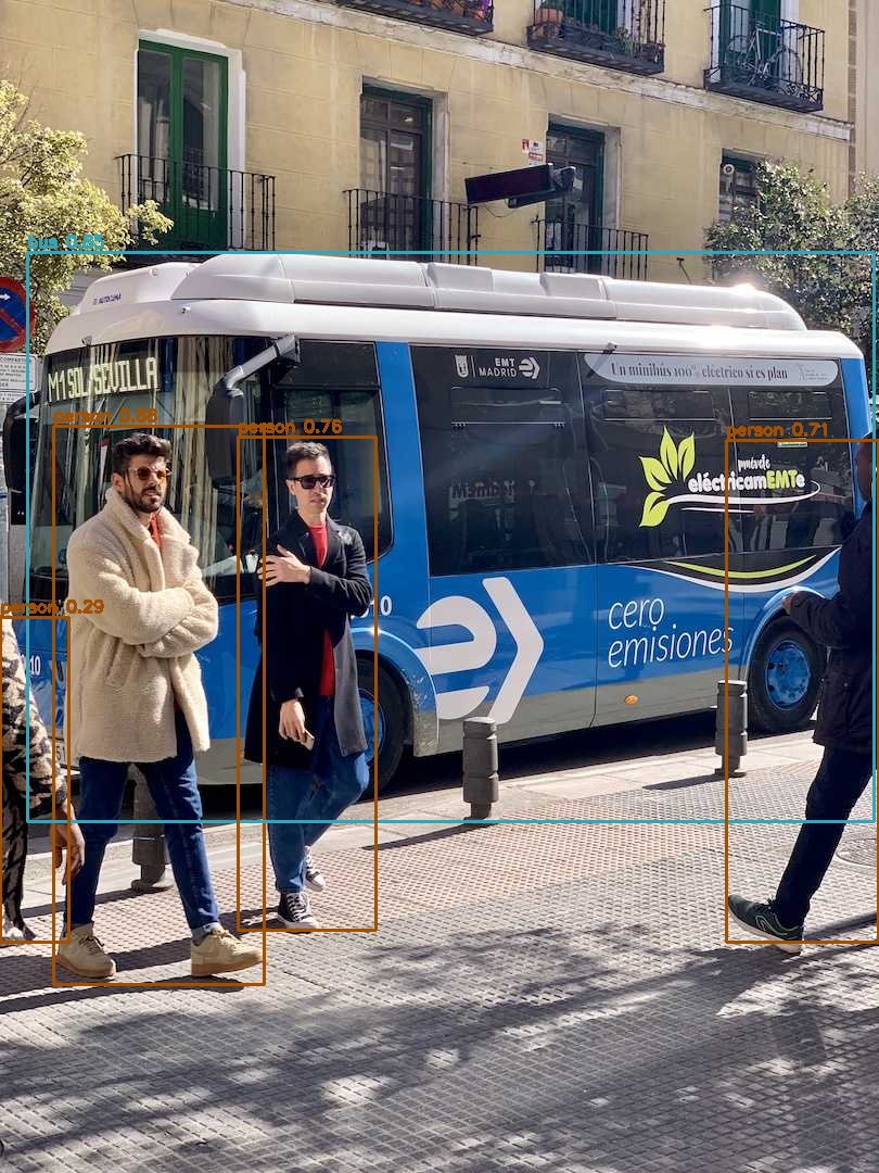
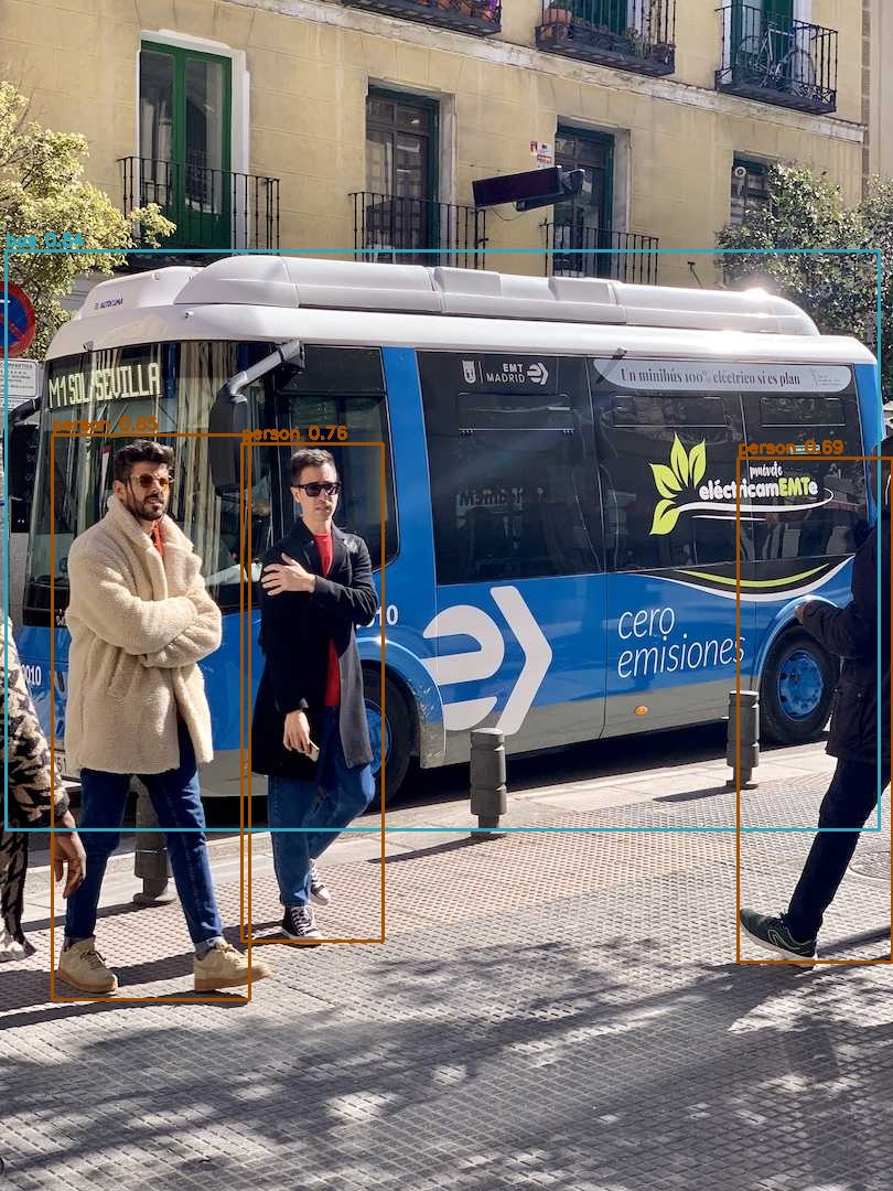
For YOLOv8n at 416 pixels, the input is [1, 3, 416, 416] and the output is [1, 84, 3549]. That is 3549 candidate boxes, each with 4 box numbers and 80 class scores, and it returns all 3549 for every single image, even a blank wall. On my test photo (figure 3), 3442 of them scored under 0.01, 43 passed the confidence threshold, and those 43 described 5 actual objects, because neighbouring grid cells all fire on the same bus.
So there is work on both sides of the model. Letterbox the photo, swap BGR to RGB, reorder HWC to CHW. Then, on the way out, filter by confidence, compute IoU, and run class-aware NMS to turn 43 candidates into 5 boxes. I wrote that in plain numpy, and on the laptop it matches the Ultralytics pipeline to three decimals on the scores and one pixel on the boxes.
On the Nano it costs this:
| Stage | Runs on | Time |
|---|---|---|
| preprocess | CPU | 12.5 ms |
| inference | GPU | 31.7 ms |
| postprocess | CPU | 6.8 ms |
| total | 51.0 ms, 19.6 FPS |
That is 38% of every frame spent in numpy on a single Cortex-A57 core. Resizing one image and filtering a table does not sound like much, until you remember that each step touches half a million numbers on a CPU that was built for a phone.
There is a second, quieter loss hiding in that table. The exact same engine takes 25.6 ms inside trtexec and 31.7 ms when I call it from my Python loop. One clue is a line in the trtexec output called Enqueue Time: about 10 ms of host-side time per frame spent submitting the inference work. trtexec can overlap that work with GPU execution. My simple synchronous loop does not. I say this is a clue rather than the answer because I did not isolate it with an experiment.
The cost of streaming a live video
Then I added the camera.
The Nano had none, so my laptop encoded its webcam as H.264 and sent it as RTP over UDP. The Nano decoded it, ran detection, drew the boxes, encoded the frame as JPEG to send back, and encoded it a second time to save a recording. All of that is CPU work. It added about 36 ms per frame.
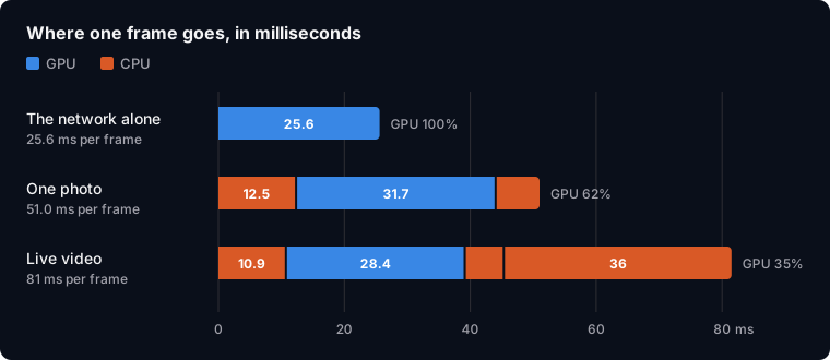
Look at the bottom bar. One frame of live video takes 81 ms, and the GPU is working for 28 of them.
The GPU was idle about two thirds of the time. The accelerator, the whole reason this board exists, was the least busy part of the system. It spent most of each frame waiting for four small ARM cores to finish shuffling pixels.
Inside the 25.6 ms
At this point the one number that still looked clean was the first one. So I opened that up too. trtexec has a profiling mode that times every layer separately.
After TensorRT’s layer fusion, the engine runs as 185 layers. Here is how the time splits:
| Kind of layer | Count | Share of GPU time |
|---|---|---|
| Convolutions | 61 | 60% |
| Activations and other pointwise layers | 62 | 21% |
| Reshape, copy, split, resize, softmax, pooling | 62 | 19% |
Convolutions are the heavy arithmetic, the part everyone pictures when they think of a CNN. They are only 60% of the time. And the slowest single layer in the entire network is not a convolution at all. It is the fused SiLU activation right after the first convolution, working on the largest feature map in the network, 16 x 208 x 208. No weights, almost no arithmetic, 5.9% of the total.
I also built a second engine at 320 pixels. That is 0.59 times as many pixels, so I expected 0.59 times the time. I got 0.66. If I model the time as a fixed part a plus a per-pixel cost b, the two measurements give two equations:
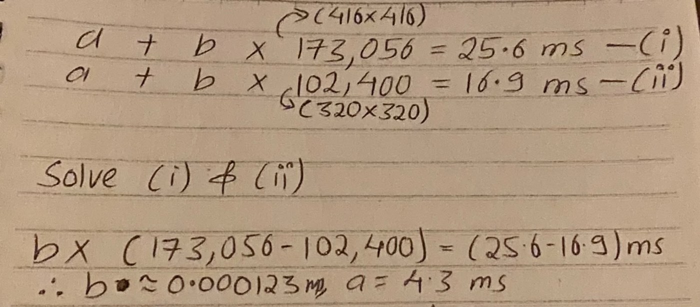
Under that model, a comes out at about 4.3 ms. Spread over 185 profiled layers, that is an effective ~23 microseconds per layer. Host-side dispatch and kernel-launch overhead are plausible contributors, but two input sizes are not enough to tell me where that fixed cost actually comes from. A third input size would have started to test the model. What the estimate does explain is why shrinking the image does not buy the full pixel-ratio speedup.
The smaller input has a price too. It is 1.5 times faster, and it loses the hardest object in the photo.
The explanation I had to throw away
FP16 can be a big win on a Jetson. Half the precision, potentially much more throughput. My FP16 engine was half the size of the FP32 one on disk, and 1.29 times faster. Even after taking out the estimated fixed 4.3 ms, the part that could have scaled only managed 1.36.
I had an explanation ready, and it sounded great. Forty percent of the time is in pointwise layers that do almost no arithmetic. Those layers must be limited by memory bandwidth, and FP16 does not help with moving data. It fit the numbers. It was in my notes. I believed it.
Then I did two lines of arithmetic.
- Halving the precision also halves the bytes moved for FP16 data. If those layers were dominated by simple DRAM traffic, that should help too. So “memory bandwidth” by itself was not a satisfying explanation.
- That slowest layer reads and writes about 2.8 MB. At 25.6 GB/s, the best-case streaming time is around 0.1 ms. I measured 1.5 ms. That does not rule out the memory system; caches, access patterns, synchronization, launch overhead and TensorRT’s implementation all matter. But it does kill the simple story that the layer is just saturating DRAM bandwidth.
So my neat explanation was too simple. I am leaving that here as an open question on purpose.
One JPEG
The assignment itself could have been done in under two hours. Understanding why the numbers behaved the way they did took most of a day.
I could have pointed the model at a picture, read “bus 0.85”, and learned one thing: the model works.
Everything worth knowing about running it on that board was in the parts the assignment left out. A model benchmark measures a much narrower slice than the application around it. What runs on an edge device is a pipeline, and on small hardware the pipeline is mostly not the network.