Observing the Probabilities
Abstract
The observations here come from a small experiment following A Neural Probabilistic Language Model (Bengio et al., 2003). In the last blog, we looked at how predicting the next word could help a model learn relationships between words. Here, I wanted to see that happen in the embedding matrix itself.
I highly suggest reading the paper or my last blog, Viewing Language Through a Probabilistic Lens, which covers the theory behind this experiment.
Seeing the C learn
Our entire corpus is:
the cat sat on the mat the dog sat on the rug
Twelve words, with 7 unique words in the vocabulary. The model uses two words of context to predict the next one, giving us 10 training examples.
$C$ is the embedding matrix. It has the shape $[V, m]$, where $V$ is the vocabulary size and $m$ is the embedding dimension. Here, that is $[7, 5]$: one row of five numbers for each word. We start by filling it with random numbers.
With those initial values, here is what the model predicts:
| Context | Expected word | Model predicts | Probability of the expected word |
|---|---|---|---|
| the cat | sat | cat | 0.001 |
| the dog | sat | the | 0.011 |
| on the | mat | the | 0.000 |
Probabilities are rounded to three decimal places. That last value is very small, rather than exactly zero.
The model has no useful representation of these words yet. To learn, it compares its predictions with the actual next words using cross-entropy loss. Backpropagation gives us the gradients, and we use them to adjust the parameters in the direction that reduces the loss. This includes the rows of $C$ used for that prediction.
Meaning, when the model gets “the cat” wrong, the numbers representing “the” and “cat” also get updated. We never tell it what a cat is. Its representation changes because it helps predict what comes next.
Let’s follow the same examples through training:
| Step | sat after “the cat” | sat after “the dog” | mat after “on the” |
|---|---|---|---|
| 0 | 0.001 | 0.011 | 0.000 |
| 10 | 0.637 | 0.286 | 0.001 |
| 25 | 0.875 | 0.840 | 0.052 |
| 50 | 0.931 | 0.940 | 0.393 |
| 1000 | 0.997 | 0.998 | 0.499 |
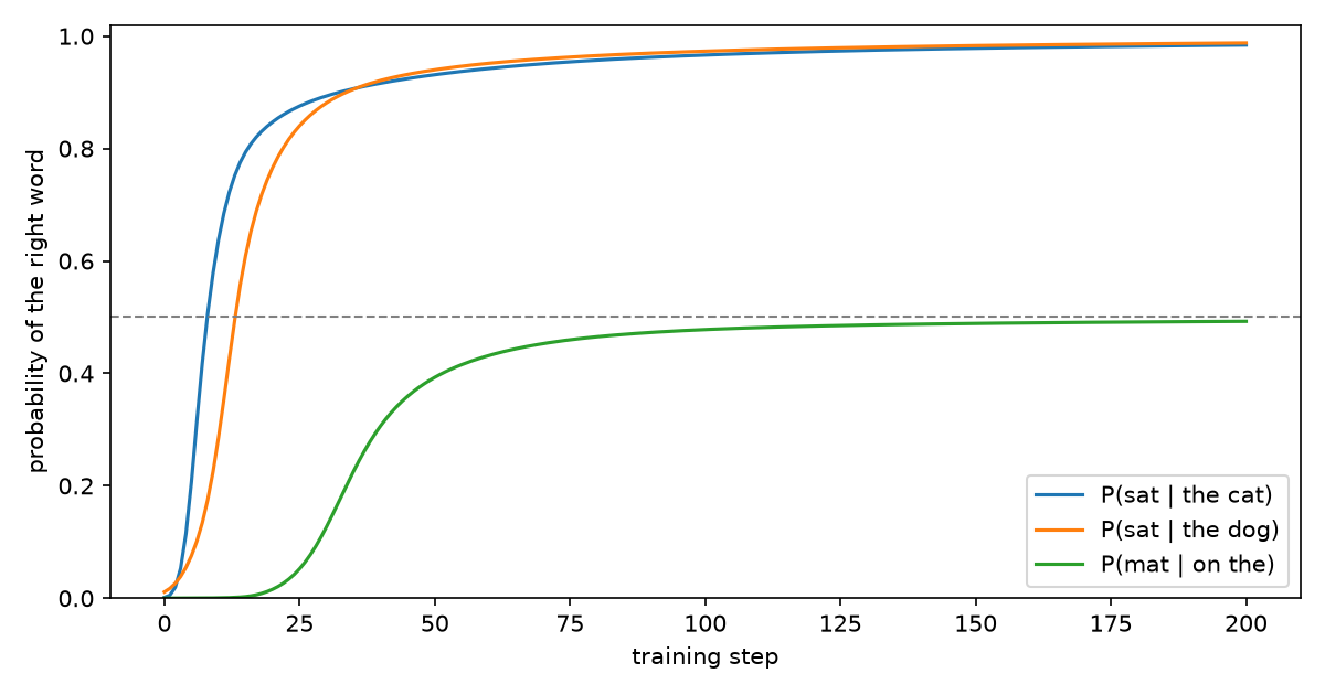
The model learns to predict sat after both “the cat” and “the dog”. But mat after “on the” only reaches about 0.5, even after 1000 steps. We will come back to why.
For this run, the embedding dimension is 5 and the hidden layer has 8 units, with the model’s direct connections enabled. I used seed 42, standard normal initialisation, and 1000 full-batch gradient descent steps at a learning rate of 0.1. The implementation is in embedding-models-from-scratch.
Chasing the cross-entropy to null
As the parameters change, the loss falls from 6.41 to 0.18 in the first 100 steps. But the remaining 900 steps only take it to 0.1415. The updates to $C$ also become much smaller.
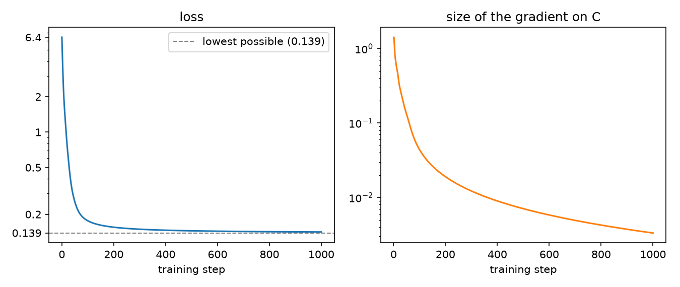
We have 256 free parameters for just 10 examples. So why does the loss stop falling?
Does a perfect model need a loss of 0?
Look at these two examples from our corpus:
on the → mat
on the → rug
The model receives exactly the same input for both. It cannot give mat a probability of 1 in one example and rug a probability of 1 in the other. Each occurs once, so the best it can do across these examples is split the probability equally.
Cross-entropy for one example is $-\ln P(\text{target})$. A probability of 1 gives a loss of 0, but a probability of 0.5 gives about 0.693. Even if the model gets the other eight examples perfectly right, the lowest average loss is:
$$ \frac{8 \times 0 + 2 \times (-\ln 0.5)}{10} \approx 0.1386 $$
Our model reaches 0.1415, already very close. And the 0.499 we saw for mat makes sense now. The model is leaving almost the other half for rug.
In natural language, this uncertainty comes up all the time. After “I drank a cup of”, the next word could be tea, coffee, milk, or water. Given only that context, there may be several valid answers. The loss left even when a model matches their probabilities is called irreducible loss, or the entropy of the next word given the context.
For our tiny corpus, the context matters quite literally. With four words instead of two, the model could distinguish “cat sat on the” from “dog sat on the”. The ambiguity disappears from these examples. So 0.1386 is the floor for this corpus with our two-word window, not a fixed limit of language.
We do not need a loss of 0 to say the model has learned these probabilities.
The relationship we wanted but couldn’t have
Normal n-gram models can predict the next word too. What interested me here was whether learning to predict would also bring related words closer together in $C$.
Cat and dog play similar roles in our corpus. So do mat and rug. We can see that when we read it, but does it show up in their representations?
I used cosine similarity to compare the rows of $C$. It measures how closely two vectors point in the same direction: 1 means the same direction, 0 means perpendicular, and -1 means opposite directions.
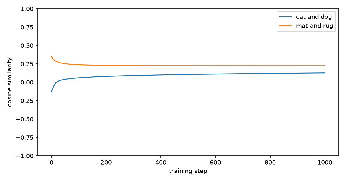
Cat and dog move a little closer, from -0.13 to 0.13. Mat and rug actually become less similar, going from 0.35 to 0.23. After training, cat’s closest word is sat, with a similarity of 0.81.
The predictions improved, but the relationships I expected were barely there.
The embedding that never learns
Rug’s row in $C$ does not change at all. After 1000 steps, its gradient is still:
[0.0, 0.0, 0.0, 0.0, 0.0]
Go back to the corpus. Rug is the last word. It appears as a target, but never as part of the context used to predict another word.
The lookup C[X] only selects rows for words in the context. Since rug is never selected, its row never receives a gradient. There is nothing updating its embedding.
The model can still learn to predict rug because the output weights are trained separately. But the row representing rug as an input stays exactly as it started. The mat/rug similarity changed only because mat moved.
Dog and cat
Cat and dog both appear in the context, and both help predict sat and on. Their embeddings do move in similar directions during training. So why do they end up only slightly closer?
They start with different random values, and the model learns these few examples before the embeddings have changed very much. As the predictions approach the best probabilities for this corpus, the overall gradient gets smaller. There is less left to update.
With 256 parameters, the model has enough room to fit these examples while keeping cat and dog quite different. Making their embeddings similar is not a separate goal in the loss function.
I also tried 10 different random seeds. The average final similarity was 0.31 for cat/dog and -0.09 for mat/rug. So changing the starting numbers did not resolve it either.
What if we add more text?
I first copied the same 10 training examples 50 times. We now have 500 examples, but the vocabulary is still 7 words, and there are still only 9 distinct context/target pairs.
| Training data | Examples | Distinct context/target pairs | cat/dog similarity | mat/rug similarity |
|---|---|---|---|---|
| Original | 10 | 9 | 0.31 | -0.09 |
| Examples copied 50 times | 500 | 9 | 0.31 | -0.09 |
These are averages over 10 seeds, with 1000 training steps per run.
No improvement. We calculate the loss as an average, so repeating every example equally leaves that average, and its gradient, unchanged. The model keeps receiving the same update at each step.
Joining the text into one long repeated string adds two contexts at the joins: “rug the” → cat and “the rug” → the. Rug finally gets used as an input, but the similarities still barely change: 0.34 for cat/dog and -0.07 for mat/rug.
We gave it more text, but almost nothing new to learn from.
What if the corpus had more combinations?
Next, I used every combination of 4 animals, 3 verbs, and 4 things in this sentence pattern:
the {cat, dog, fox, cow} {sat, lay, slept} on the {mat, rug, sofa, bed} .
That gives us 48 sentences and a vocabulary of 14 tokens, including the full stop. The full stop also means rug can now appear in a context before the sentence ends.
I kept out the 8 sentences containing “fox slept” or “cow lay”, and trained on the other 40. The model sees all the words during training, but not those combinations. The held-out loss measures how well it predicts on the sentences we kept aside. Lower is better.
For this larger corpus, I trained for 3000 steps per run. These results, and the remaining comparisons, are averages over 10 seeds.
| cat/dog similarity | mat/rug similarity | Training loss | Held-out loss |
|---|---|---|---|
| 0.69 | 0.54 | 0.529 | 1.240 |
Now the relationships are more visible. Cat and dog become much closer, and mat and rug improve too.
But the model still does much better on the sentences it trained on. The training loss is almost at this corpus’s floor of 0.526, while the held-out loss is 1.240. More combinations helped, but there is still room to improve on the unseen sentences.
What if the model had less capacity?
I reduced the embedding dimension from 5 to 2 and the hidden layer from 8 units to 4. On the larger vocabulary, that takes the model from 424 parameters to 174. The corpus and training steps stay the same.
| Model | cat/dog similarity | mat/rug similarity | Training loss | Held-out loss |
|---|---|---|---|---|
| Original size | 0.69 | 0.54 | 0.529 | 1.240 |
| Smaller | 0.94 | 0.92 | 0.536 | 0.872 |
Both pairs become much closer, and the held-out loss falls. The smaller model fits the training examples slightly less well, but does better on the sentences it has never seen.
Reducing the size does not guarantee similar embeddings. In this experiment, though, giving the model less room to fit each combination separately helped it learn representations that worked across the combinations.
What if we add weight decay?
The paper uses weight decay, which I had left out of this setup. I added it to the original-sized model on the larger corpus.
Weight decay adds a penalty for large parameter values. Here, that penalty is $\lambda$ times the sum of squared values in $C$, $H$, $U$, and $W$. The biases are left out, and $\lambda$ controls how strong the penalty is.
| Weight decay | cat/dog similarity | mat/rug similarity | Training loss | Held-out loss |
|---|---|---|---|---|
| None | 0.69 | 0.54 | 0.529 | 1.240 |
| 0.001 | 0.83 | 0.69 | 0.542 | 0.937 |
| 0.01 | 1.00 | 1.00 | 0.670 | 0.724 |
The losses shown here are cross-entropy alone, without the added penalty, so we can compare them with the previous runs.
At 0.01, the paired embeddings point in almost the same direction. This setting also gives the lowest held-out loss of the ones I tried, even though its training loss is higher.
That makes sense for the corpus we built. Every animal and every thing can occupy its group’s slot in the sentence. Real language has more differences to preserve. Cat and dog having almost identical directions here does not mean that should be our goal for every corpus.
Conclusion
In our previous blog, we covered the architecture and tried understanding the underlying mechanism. In this blog, I tried running it. This is not the current state-of-the-art model, and it is way behind the frontier. The purpose of the blog was to understand how complex relationships are learned and represented in vectors.
While the world is busy chasing the frontier, I think understanding its foundations is just as important. The purpose of this blog and the entire series is to build intuition. In a way, I am trying to build my own embedding matrix $C$ such that I start building the correct research intuition.