ELMo: From One Word Vector to Context
Preface
From NPLM and Word2vec to GloVe, we always had one fixed input vector for a word, meaning the word “bank” was not easily separable by whether the context it was being used in was related to money or to a river. This is the one core problem that we have to follow through this entire blog.
P.S. in this blog we will cover some new concepts, followed by experiments and observations that I encountered. If you already know these concepts, you can move straight to the experiments.
Character convolution
Word2vec and GloVe learn word relationships from the contexts in which words occur. But each word has its own vector, so rare words have limited evidence, and unseen words have no learned vector.
A character CNN instead constructs a word’s representation from its spelling. For example, a width-three filter examines character sequences such as sin and ing in sing. The same filter is applied across other words, allowing training to discover reusable spelling patterns. These patterns need not correspond to complete words or meaningful word parts.
Each filter scores the character windows it examines. Max-pooling keeps its strongest score across the word. We collect one score per filter, then process them into one word vector. So the LSTM receives whole-word vectors, not separate vectors for sin and ing.
This lets information learned from familiar words contribute to representations of rare or unseen words. The character CNN captures information from spelling; ELMo’s later LSTM layers incorporate the surrounding sentence.
The problem with a simple RNN
A simple RNN reads one token at a time, combining it with the previous hidden state to produce a new one:
$$ h_t = \tanh(W_x x_t + W_h h_{t-1} + b) $$
Here, $x_t$ represents the current token, and $h_{t-1}$ is the summary of what came before. The weights and bias are learned during training.
Consider:
Pragalva, who spends his evenings reading research papers and writing blog posts, is learning about ELMo.
When predicting “is,” the RNN needs information about the singular subject “Pragalva.” But that information must survive every hidden-state update while the model reads the intervening words. Each update rewrites the summary, potentially weakening or overwriting what matters.
Training has a related difficulty. If the model incorrectly predicts “are,” the correction signal must travel backward through those updates. Repeated multiplication by small factors can make that signal tiny: shrinking it by half ten times leaves less than one-thousandth of its original size. This is the vanishing-gradient problem, which makes long-distance dependencies difficult to learn.
LSTM: deciding what to remember
In a simple RNN, the hidden state is repeatedly rewritten. LSTM introduces a separate memory cell, $c_k$, with gates that control its updates:
-
Forget gate, $f_k$: how much existing memory to retain.
-
Input gate, $i_k$: how much proposed new information to add.
-
Output gate, $o_k$: how much of the updated memory to expose through the hidden state.
The memory update is:
$$ c_k = f_k \odot c_{k-1} + i_k \odot \tilde{c}_k $$
Here, $\tilde{c}_k$ is the proposed new information, and $\odot$ means multiplying corresponding components.
In our sentence about Pragalva reading papers, the model can learn to retain information about the subject while processing the intervening words. If a forget-gate component stays near 1, that part of the memory passes forward with little change. This also gives the training signal a path that helps reduce the vanishing-gradient problem.
Bidirectional LSTM
LSTM helps retain information, but reading direction matters too. Consider:
I visited the bank to deposit money.
I visited the bank to sit beside the river.
The words before “bank” are identical. A forward LSTM has the same information at that position in both sentences. The words that clarify the meaning come afterward.
ELMo uses two LSTM stacks:
-
A forward stack reads left to right and learns to predict the next token.
-
A backward stack reads right to left and learns to predict the previous token.
Each direction has two stacked LSTM layers. The second layer processes the first layer’s outputs, adding another stage of computation without changing the reading direction.
At each word and each LSTM level, we concatenate the forward and backward hidden-state vectors, placing them side by side. The representation of “bank” now includes information from both the preceding and following text.
Word2vec and GloVe can use surrounding words on both sides during training, but their learned word embeddings remain fixed across sentences. ELMo computes a representation for each occurrence, allowing the same word to receive different vectors depending on its context.
Combining the layers
For each word occurrence, we now have three representations:
| Layer | What it contains |
|---|---|
| 0 | The character-based word vector, without sentence context |
| 1 | The first LSTM layer’s forward and backward vectors, joined |
| 2 | The second LSTM layer’s forward and backward vectors, joined |
During language-model training, the top forward output predicts the next whole word, and the top backward output predicts the previous word. Softmax turns vocabulary scores into probabilities. The prediction error trains the character CNN and LSTMs together.
For a new task, ELMo blends the three representations using learned weights:
$$ v = \gamma(s_0h_0 + s_1h_1 + s_2h_2) $$
The weights add up to 1, and $\gamma$ scales the blend. Our experiment normalizes the layers before mixing to account for their different scales.
This part took me a while to picture: we freeze the language model, save its output vectors, and train a new mixture and classifier on those numbers. The old weights stay unchanged. We learn how to use its outputs, rather than fine-tuning the network itself.
Experiments
This was our first long GPU run in this series, on a corpus of roughly 100 million words. The notebook was put together with assistance; my goal here is to understand what the run did and what its results actually tell us.
We trained a smaller ELMo-style model on WikiText-103, a collection of Wikipedia text:
| Run detail | Value |
|---|---|
| GPU | NVIDIA A100, 40 GB |
| Training corpus | 101,425,671 words |
| Model | About 26.9 million parameters |
| Training | 10 passes, 123,810 update steps |
| Recorded training time | 2.58 hours, excluding evaluation and setup |
Ten passes mean roughly a billion word-position exposures, not a billion distinct words. Our model and corpus are smaller than the paper’s, so its benchmark is not directly comparable.
Did it learn to predict words?
We tested on text excluded from training. Perplexity measures prediction uncertainty: lower means more probability assigned to the actual words. It is not an accuracy percentage.
| Model | Test perplexity |
|---|---|
| Word-frequency baseline, ignoring context | 1211.1 |
| Trained forward language model | 51.5 |
| Trained backward language model | 51.5 |
Context helped prediction substantially, and both directions performed almost identically.
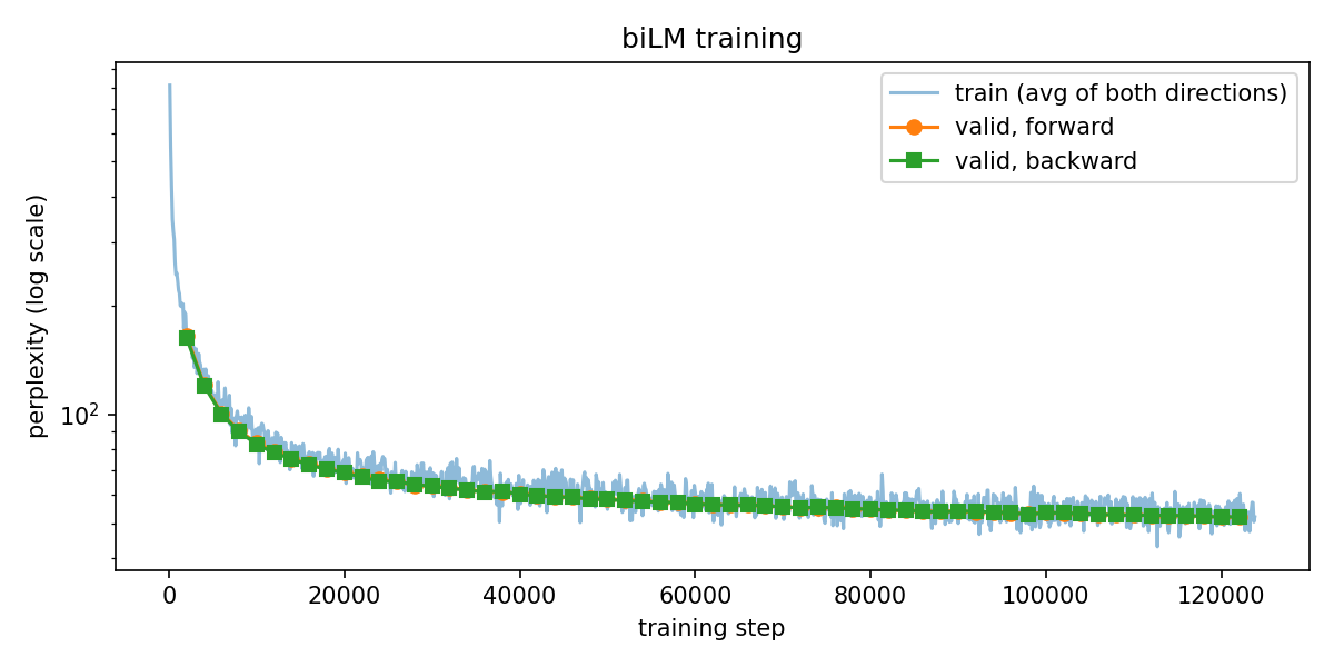
Training and validation perplexity fall together, then improvement slows.
Did “bank” split by meaning?
Finally, the question that started this blog gets a test. We used bank, plant, and cell, with two meanings each: 24 sentences total.
For each occurrence, we found the closest other representation of that same word using cosine similarity. Did the neighbour use the same meaning?
| Representation | Trained model | Untrained model |
|---|---|---|
| Layer 0 | Cannot separate meanings | Cannot separate meanings |
| Layer 1 | 70.8% | 54.2% |
| Layer 2 | 87.5% | 54.2% |
Layer 0 gives the same word the same vector in every sentence, so every comparison ties. The code reports 50% because it picks the first neighbour when scores tie; that number does not measure meaning separation. Layer 2 matched the meaning in 21 of 24 cases.
Even random LSTMs produce vectors that change with context. Different vectors alone are not enough; training should make those differences useful. The trained model grouped meanings better, but 24 examples do not establish that every ambiguous word is solved.
Can other tasks use these representations?
We froze the language model and trained small classifiers for two tasks: positive or negative sentiment, and part-of-speech tagging, such as noun or verb. Each task used a small linear classifier on the frozen vectors, rather than the paper’s full task model, so the accuracies are not directly comparable. For sentiment, we averaged the vectors over the sentence; for grammar, we classified each word. We compared using one layer with learning a mixture of all three.
| Representation | Sentiment accuracy | Part-of-speech accuracy |
|---|---|---|
| Layer 0 only | 71.0% | 92.6% |
| Layer 1 only | 74.7% | 96.3% |
| Layer 2 only | 78.4% | 96.3% |
| Learned mixture | 78.7% | 96.5% |
| Learned mixture from an untrained model | 62.0% | 78.2% |
Sentiment used 20,000 SST-2 training examples and was evaluated on its public validation set. Grammar used an 80/20 sentence split of the Penn Treebank sample.
The sentiment mixture put about 86% of its weight on layer 2. The grammar mixture spread its weights more: about 15%, 35%, and 49% across layers 0, 1, and 2. These were learned for each task, not separately for each word. Our grammar result did not show a clear win for layer 1 over layer 2.
Using the rounded table values, the mix added 0.3 percentage points for sentiment and 0.2 for grammar. The gains from the unrounded scores were 0.23 and 0.19 points, respectively. Pretraining raised sentiment accuracy from 62.0% to 78.7%, and grammar accuracy from 78.2% to 96.5%. That was the bigger difference in this run. A single run cannot tell us much about the small gain from mixing layers.